20

Overview

In my first ever #tidytuesday we are taking a look at a coffee survey. I’ll make a note up front that I am prioritizing self education over analytical integrity here. Curiosity is in the drivers seat, so we are going to see where this takes us. Anything I present here is not intended to draw any conclusions or correlations (I tried, and any statistically sound correlation just wasn’t there with this data).

ELT

Load Up

Nothing crazy.

library(tidytuesdayR)
library(tidyverse)
library(RColorBrewer)
library(ggforce)
library(knitr)
library(kableExtra)

Theme Setup

Coffee Colors?

brew_colors <- brewer.pal(n = 6, name = "YlOrBr")

coffee_theme <- theme_minimal() +
  theme(
    plot.title = element_text(family = "Hot Ink", face = "plain", size = 26, color = brew_colors[1], hjust = 0.5),
    axis.title.x = element_text(family = "Fira Sans", face = "italic", size = 12, color = brew_colors[1], margin = margin(t = 20, r = 20, b = 20, l = 20, unit = "pt")),
    axis.title.y = element_text(family = "Fira Sans", face = "italic", size = 12, color = brew_colors[1], margin = margin(t = 20, r = 20, b = 20, l = 20, unit = "pt")),
    axis.text.x = element_text(family = "Fira Sans", face = "plain", size = 10, color = brew_colors[2], angle = 45, hjust = 1),
    axis.text.y = element_text(family = "Fira Sans", face = "plain", size = 10, color = brew_colors[2]),
    legend.title = element_text(family = "Fira Sans", face = "bold", size = 12, color = brew_colors[1]),
    legend.text = element_text(family = "Fira Sans", face = "plain", size = 10, color = brew_colors[2]),
    plot.background = element_rect(fill = "black", color = NA),
    panel.background = element_rect(fill = "black", color = NA),
    panel.grid.major = element_blank(),
    panel.grid.minor = element_blank(),
    plot.margin = margin(t = 35, r = 10)
  )

theme_set(coffee_theme)

Extract

I tried the tidytuesdayR::tt_load method and kept getting an error, so we url it.

coffee_survey <- read_csv('https://raw.githubusercontent.com/rfordatascience/tidytuesday/master/data/2024/2024-05-14/coffee_survey.csv', show_col_types = FALSE)

Transform

Nice initial cleaning. I decided straight away that my analysis would not be considering open-response answers. I organized the rest of the columns into two categories: multiple response, and factored. Here I factor the latter group. Later I’ll decide what to do with the former.

Finally I have the pleasure of correcting the “spend” column typo. People need to stop using “spend” as a noun. It is a verb. The noun is “expenditure”.

# Trim out free-text data, fix "spend" typo 
# "spend" is not a noun, stop trying to make it one
clean_tib <- coffee_survey %>%
  select(-matches("other|specify|coffee_a|coffee_b|coffee_c|coffee_d|prefer")) %>%
  rename(monthly_expenditure = total_spend) %>%
  mutate(across(everything(), ~ if(is.character(.)) tolower(.) else .)) %>%
  mutate(across(c(age, cups, favorite, style, strength, roast_level, caffeine,
                  expertise, wfh, monthly_expenditure, taste, know_source,
                  most_paid, most_willing, value_cafe, spent_equipment,
                  value_equipment, gender, education_level, ethnicity_race,
                  employment_status, number_children, political_affiliation
                  ), as.factor
                )
         )

EDA

I saw the multiple-response columns and decided to try to learn more about the best ways to handle these. I could make each cell a vector, turning the column into a list of character vectors, or I could try one-hot encoding. I brought in the caret library and played around with dummy variables enough to get a basic transformation of all the multiple-response columns into multiple single Boolean columns for each response.

This was messy and I didn’t love my function but it was enough to try some Chi Square/Cramérs V analysis comparing every column pair for possible correlation. I would love to have found ANY surprise coffee trend that correlated to personal data (like maybe all the cinnamon takers are all unemployed), but the highest Cramérs V value was .5 and nothing compelling. So I gave up before I started showing more bias than I had already in wanting to find something.

I may clean that code up and include it later.

Strip Columns

But for now I stripped out all of those multiple-response columns. This allowed me to drop all NA cells. These columns were the questions that many people seem to have just skipped, so stripping them saved more observations.

# List of columns with multi-value cells
hot_columns <- c("where_drink",
                 "brew",
                 "purchase",
                 "additions",
                 "dairy",
                 "sweetener",
                 "why_drink"
                 )

# Drop multi-value columns before dropping NA cells
strip_tib <- clean_tib %>%
  select(-all_of(hot_columns)) %>%
  drop_na()

First Plot

I wanted to plot some kind of two-variable comparison anyway so I chose Age vs Cups per day, just to have a look.

# Ordinal ordering
age_levels = c("<18 years old", "18-24 years old", "25-34 years old",
               "35-44 years old", "45-54 years old", "55-64 years old",
               ">65 years old")
cups_levels = c("less than 1", "1", "2", "3", "4", "more than 4")

ageVcups <- strip_tib %>% 
  select(age, cups) %>% 
  mutate(
    age = factor(age, levels = age_levels, ordered = TRUE),
    cups = factor(cups, levels = cups_levels, ordered = TRUE)
  )

ggplot(ageVcups, aes(x = age, fill = cups)) +
  geom_bar(
    position = "fill"
    ) +
  labs(
    title = "Cups of Coffee per Day by Age Group",
    x = "Age Group",
    y = "Percentage",
    fill = "Number of Cups"
    ) +
  scale_fill_brewer(
    palette = "YlOrBr"
    ) +
  scale_y_continuous(
    labels = ~ paste0(. * 100, "%")
    ) +
  theme(
    legend.position = "right",
    axis.text.x = element_text(angle = 45, hjust = 1)
  )

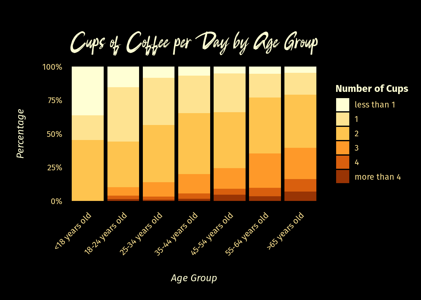
No considerable surprise that older age groups tend to show a greater proportion of higher cups-per-day.

Finding Our Target

What interested me is the self-reported coffee expertise. These questions are such a labyrinth of psychology I don’t know what analysts really use them for other than profiling over confidence maybe? I thought Dunning-Kruger did away with the presumed value of self-assessed expertise.

What other question might be fun to compare to this self-expertise?

“Do you know the source of your coffee”

Lets take a look. A jitter-box plot will show this nicely.

expertiseVknowsource_tib <- strip_tib %>%
  select(expertise, know_source) %>% 
    mutate(know_source = case_when(
      tolower(know_source) == "yes" ~ "Yes",
      tolower(know_source) == "no" ~ "No",
      TRUE ~ know_source))

evk_lite <- expertiseVknowsource_tib %>% 
  filter(!(know_source == "No" & expertise == 10))

evk_hilite <- expertiseVknowsource_tib %>% 
  filter(know_source == "No" & expertise == 10)

p <- ggplot(evk_lite, aes(
    x = know_source, 
    y = as.numeric(expertise))
  ) +
  geom_boxplot(
    data = expertiseVknowsource_tib,
    outlier.shape = NA, 
    fill = "brown", 
    color = "white", 
    alpha = 0.25
  ) +
  geom_point(
    data = evk_lite,
    position = position_jitter(seed = 119, width = 0.12, height = 0.69),
    color = "tan",
    alpha = 0.25
  ) +
  geom_point(
    data = evk_hilite,
    position = position_jitter(seed = 119, width = 0.1, height = 0.69),
    color = "tan",
    alpha = 0.25
  ) +
  scale_y_continuous(
    breaks = seq(0, 10, by = 1)
  ) +
  labs(
    title = "Do Coffee Experts Know Their Sources?",
    x = "Do You Know Where Your Coffee Comes From?",
    y = "Claimed Level of Coffee Expertise"
  ) +
  theme(
    legend.position = "none"
  )

p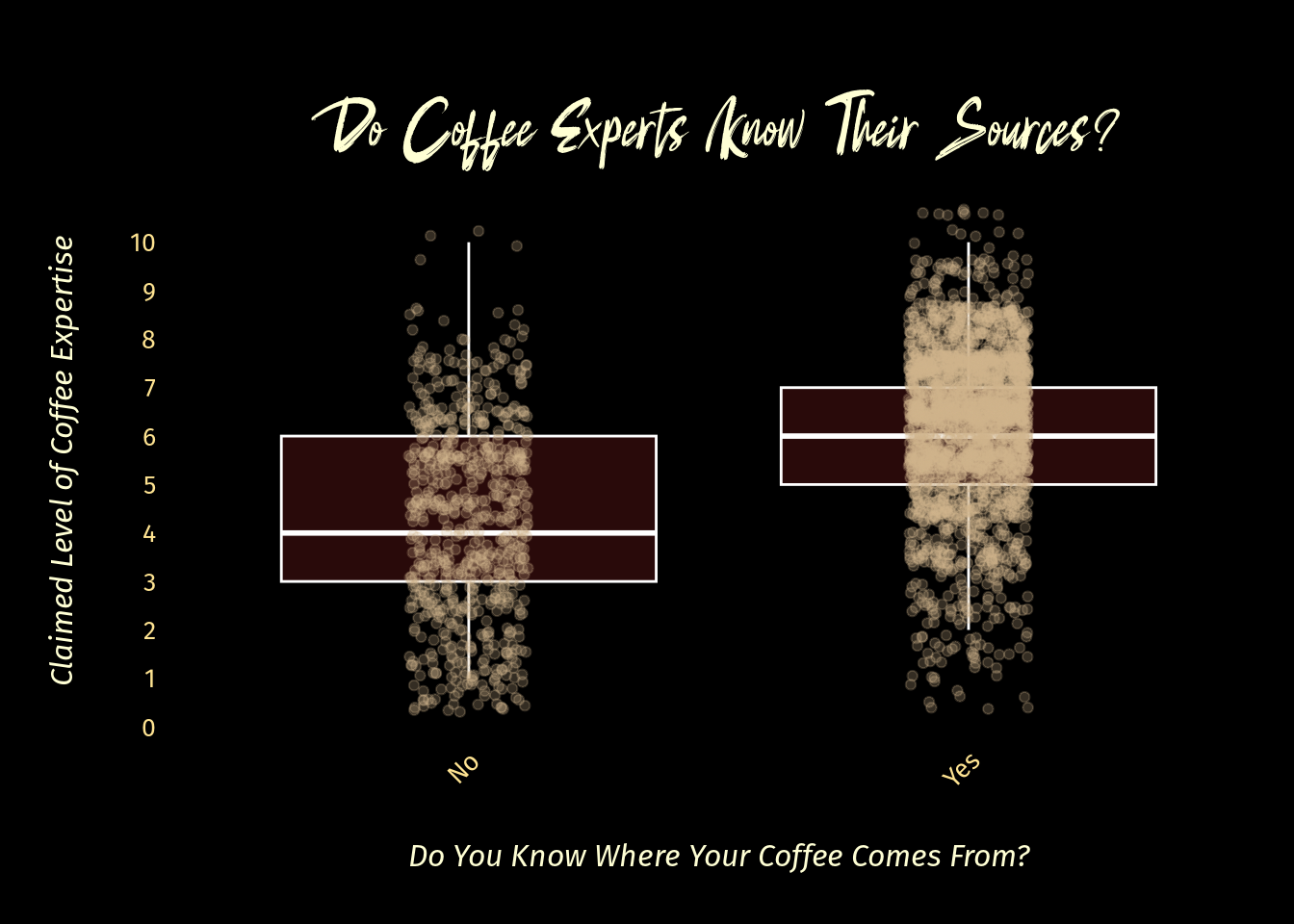

Results

Not too suprising. The more you claim to know about coffee the more likely you are to also claim to know where your coffee comes from.

But who are those four coffee geniuses who don’t care where their coffee comes from?

hilite <- expertiseVknowsource_tib %>% 
  filter(know_source == "No" & expertise == 10)

# set.seed(357)
# jitter <- position_jitter(width = 0.25, height = 0.5)

p_hilite <- p +
  geom_point(data = hilite, aes(
    x = know_source, 
    y = as.numeric(expertise)),
    position = position_jitter(seed = 119, width = 0.1, height = 0.69), 
    color = "brown",
    alpha = .88
    ) +
  annotate(
    "text",
    x = .75,
    y = 10,
    label = "EXPERTS",
    size = 2.5,
    #fontface = "italic",
    color = "brown"
  )

p_hilite

Drill Down

I must know more about them

expVsource_outliers <- strip_tib %>%
  mutate(expertise = as.integer(expertise)) %>%
  select(-submission_id) %>% 
  filter(expertise == 10) %>%
  filter(str_detect(know_source, "no"))


kable(expVsource_outliers, "html") %>%
  kable_styling() %>%
  row_spec(0, bold = TRUE, color = brew_colors[1], background = "brown") %>%
  row_spec(1:nrow(expVsource_outliers), color = brew_colors[6], background = brew_colors[1])

age	cups	favorite	style	strength	roast_level	caffeine	expertise	wfh	monthly_expenditure	taste	know_source	most_paid	most_willing	value_cafe	spent_equipment	value_equipment	gender	education_level	ethnicity_race	employment_status	number_children	political_affiliation
18-24 years old	2	americano	caramalized	very strong	light	full caffeine	10	i primarily work from home	<$20	yes	no	$6-$8	$4-$6	yes	$100-$300	yes	female	bachelor's degree	asian/pacific islander	employed full-time	none	no affiliation
25-34 years old	1	regular drip coffee	chocolatey	somewhat strong	dark	full caffeine	10	i primarily work from home	$40-$60	yes	no	$10-$15	$15-$20	yes	$20-$50	yes	female	bachelor's degree	asian/pacific islander	employed full-time	none	no affiliation
18-24 years old	1	latte	chocolatey	very strong	medium	full caffeine	10	i primarily work in person	$60-$80	yes	no	$6-$8	$6-$8	yes	$50-$100	yes	female	bachelor's degree	asian/pacific islander	employed full-time	none	independent
25-34 years old	1	pourover	chocolatey	somewhat strong	dark	full caffeine	10	i primarily work from home	<$20	yes	no	$8-$10	$10-$15	yes	$300-$500	yes	male	bachelor's degree	white/caucasian	employed full-time	none	independent

Responsible Analysis

Let’s remind ourselves that we left sound analysis practices behind at this point. We are simply having fun. These are outliers and ZERO conclusions can be drawn from digging into their data. So lets just stop here.